The Whiz and Viz Bang of Data

class: center, middle, inverse, title-slide

.title[
# The Whiz and Viz Bang of Data
]
.subtitle[
## The Basics of Visualizaiton and Modeling
]
.author[
### Dr. Christopher Kenaley
]
.institute[
### Boston College
]
.date[
### 2026/9/21
]

---

# In class today

<link rel="stylesheet" href="https://cdnjs.cloudflare.com/ajax/libs/font-awesome/5.14.0/css/all.min.css">

.pull-left[
Today we'll ....

- Look at some models

- Choose which models fit best

- Peak under the hood of Module Project 3

Next time . . .

- Account for phylogenetic history

]

.pull-right[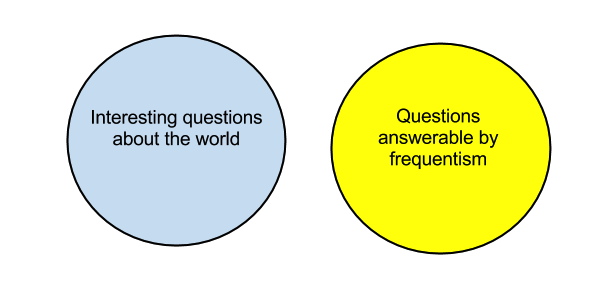
![](https://cxl.com/wp-content/uploads/2015/08/bayesian2.png)
]

---

# What is a model?

- a mathematical explanation of a process or system

- Predictions in R: `y~x`

- but can me more complex:

* `y~x+a`
  * `y~x+a+b`
  * `y~x+a+b+c`
  * etc.
  
- Linear model: `lm(y~x)`

* But could be some other model

---

# What is a model?

.pull-left[

``` r
set.seed(123)
x_A=1:50
y_A=x_A*2+runif(50,1,200)
x_B=1:50
y_B=x_B*3.5+runif(50,1,200)

d <- tibble(x=c(x_A,x_B),
            y=c(y_A,y_B),
            species=c(rep("A",50),
                      rep("B",50))
            )
```
]

.pull-right[

``` r
d%>%
  ggplot(aes(x,y,col=species))+
  geom_point()+
  geom_smooth(method="lm")
```

![](3140_f26_9-21_files/figure-html/unnamed-chunk-3-1.png)
]
---

# Approach 1: Do the data adhear to an *a priori* model?

The frequentist approach

``` r
fit_1 <- lm(y~x,data=d)

anova(fit_1)
```

```
## Analysis of Variance Table
## 
## Response: y
##           Df Sum Sq Mean Sq F value   Pr(>F)    
## x          1 103506  103506  28.016 7.36e-07 ***
## Residuals 98 362063    3695                     
## ---
## Signif. codes:  0 '***' 0.001 '**' 0.01 '*' 0.05 '.' 0.1 ' ' 1
```

---

# Approach 1: Do the data adhear to an *a priori* model?

The frequentist approach

``` r
summary(fit_1)
```

```
## 
## Call:
## lm(formula = y ~ x, data = d)
## 
## Residuals:
##      Min       1Q   Median       3Q      Max 
## -115.619  -47.956   -1.212   54.139  130.530 
## 
## Coefficients:
##             Estimate Std. Error t value Pr(>|t|)    
## (Intercept) 113.4884    12.3412   9.196 6.73e-15 ***
## x             2.2294     0.4212   5.293 7.36e-07 ***
## ---
## Signif. codes:  0 '***' 0.001 '**' 0.01 '*' 0.05 '.' 0.1 ' ' 1
## 
## Residual standard error: 60.78 on 98 degrees of freedom
## Multiple R-squared:  0.2223,	Adjusted R-squared:  0.2144 
## F-statistic: 28.02 on 1 and 98 DF,  p-value: 7.36e-07
```

---

# Approach 1: Do the data adhear to an *a priori* model?

The frequentist approach

.pull-left[

``` r
fit_2 <- lm(y~x+species,d)
anova(fit_2)
```

```
## Analysis of Variance Table
## 
## Response: y
##           Df Sum Sq Mean Sq F value    Pr(>F)    
## x          1 103506  103506 29.5261 4.099e-07 ***
## species    1  22023   22023  6.2823   0.01386 *  
## Residuals 97 340040    3506                      
## ---
## Signif. codes:  0 '***' 0.001 '**' 0.01 '*' 0.05 '.' 0.1 ' ' 1
```
]

---

# Approach 1: Do the data adhear to an *a priori* model?

The frequentist approach

.pull-left[

``` r
fit_3 <- lm(y~x*species,d)
anova(fit_3)
```

```
## Analysis of Variance Table
## 
## Response: y
##           Df Sum Sq Mean Sq F value    Pr(>F)    
## x          1 103506  103506  32.631 1.247e-07 ***
## species    1  22023   22023   6.943  0.009812 ** 
## x:species  1  35530   35530  11.201  0.001168 ** 
## Residuals 96 304510    3172                      
## ---
## Signif. codes:  0 '***' 0.001 '**' 0.01 '*' 0.05 '.' 0.1 ' ' 1
```
]

---

# Approach 1: Do the data adhear to an *a priori* model?

Which model do we use?

``` r
lapply(list(fit_1,fit_2,fit_3),
       function(x) setNames(anova(x)$`Pr(>F)`,rownames(anova(x))))
```

```
## [[1]]
##            x    Residuals 
## 7.360104e-07           NA 
## 
## [[2]]
##            x      species    Residuals 
## 4.099474e-07 1.385842e-02           NA 
## 
## [[3]]
##            x      species    x:species    Residuals 
## 1.246589e-07 9.811668e-03 1.168171e-03           NA
```

---

#Approach 2: Are models accurate descriptions of the data?

## Information theory
.pull-left[

- What is the likelihood that the model fits the data?
  - Treat each model like an hypothesis about the process.
  - Find the model that explains the data best.

>Likelihood (aka, likelihood function):  How well does a statistical model explain observed data by calculating the probability of seeing that data under different parameter values of the model?

``` r
sapply(list(fit_1,fit_2,fit_3),
       logLik)
```

```
## [1] -551.6140 -548.4763 -542.9583
```

]

.pull-right[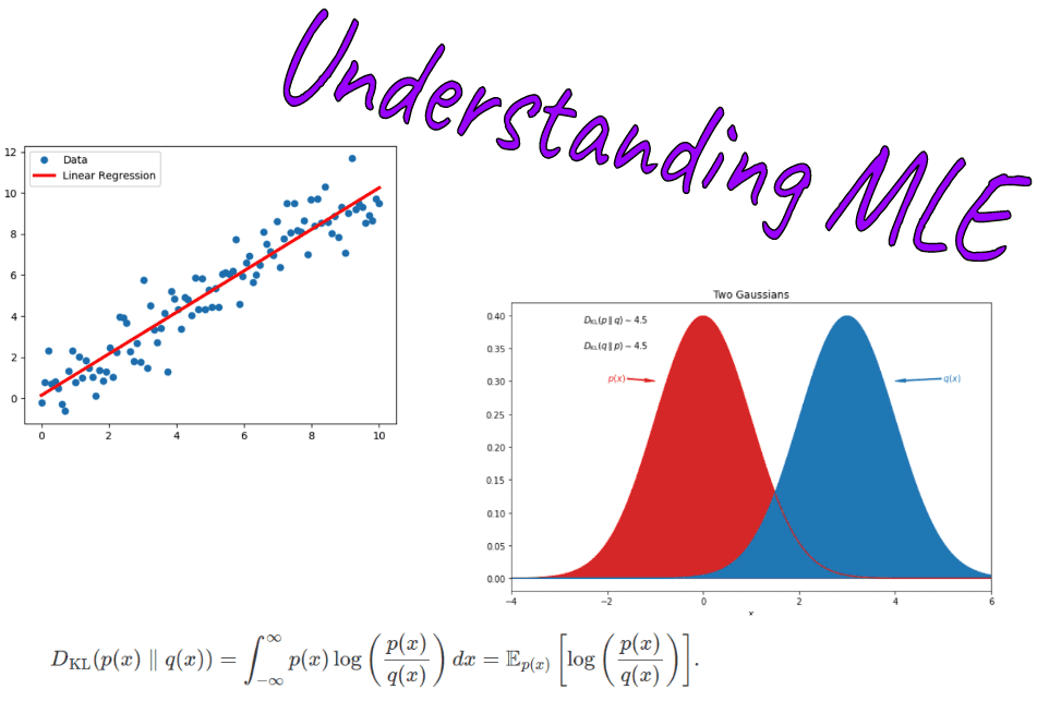
![](
https://theaisummer.com/static/052160ea37856767a70d005c35651c01/8d2ee/mle.png)
]

---

#Approach 2: Are models accurate descriptions of the data?

## Information theory
.pull-left[

- What is the likelihood that the model fits the data?
  - Treat each model like an hypothesis about the process.
  - Find the model that explains the data best.

In regression models, we're asking . . .

>If the slope, intercept, and residual variance had these particular values, how plausible would my observed cloud of points be?

``` r
sapply(list(fit_1,fit_2,fit_3),
       logLik)
```

```
## [1] -551.6140 -548.4763 -542.9583
```

]

.pull-right[
![](
https://theaisummer.com/static/052160ea37856767a70d005c35651c01/8d2ee/mle.png)
]

---

#Approach 2: Are models accurate descriptions of the data?

## Information theory
.pull-left[

- What is the likelihood that the model fits the data?
  - Treat each model like an hypothesis about the process.
  - Find the model that explains the data best.

The likelihood function is the model’s compatibility score for different parameter values, judged against the data you actually observed.

``` r
sapply(list(fit_1,fit_2,fit_3),
       logLik)
```

```
## [1] -551.6140 -548.4763 -542.9583
```

]

.pull-right[
![](
https://theaisummer.com/static/052160ea37856767a70d005c35651c01/8d2ee/mle.png)
]

---

#Approach 2: Are models accurate descriptions of the data?

## Information theory
.pull-left[
  - What is the likelihood that the model fits the data?
  - Treat each model like an hypothesis about the process.
  - Find the model that explains the data best **accounting for the number of parameters**.

AIC: does any one model fit the data best given the number of parameters?

``` r
AIC(fit_1,fit_2,fit_3)
```

```
##       df      AIC
## fit_1  3 1109.228
## fit_2  4 1104.953
## fit_3  5 1095.917
```

]

.pull-right[
![](https://timeseriesreasoning.files.wordpress.com/2021/06/a6352-1nurn_wtjfpwin0mc6t7myq.png)
]